Tympan with an HDA 200 Headset

When using a device like the Tympan for hearing science, it is important to know the maximum loudness that can be produced by your system. If you cannot get loud enough, it can limit the range of hearing loss that you can work with. It is important to know how loud you can get. So, we measured the maximum sound pressure level that can be produced by the Tympan when used with a standard HDA 200 headset from Sennheiser. Let’s see what it can do!

GOAL

Our goal was to measure the maximum sound pressure level (SPL) that the Tympan can produce when driving an HDA200 headset without generating excessive harmonic distortion.

APPROACH

We measured the output of the HDA200 using an artificial ear.  We had the Tympan generating test tones at increasing loudness until either (1) we exceeded our self-imposed limit on harmonic distortion or (2) the Tympan could go no louder.

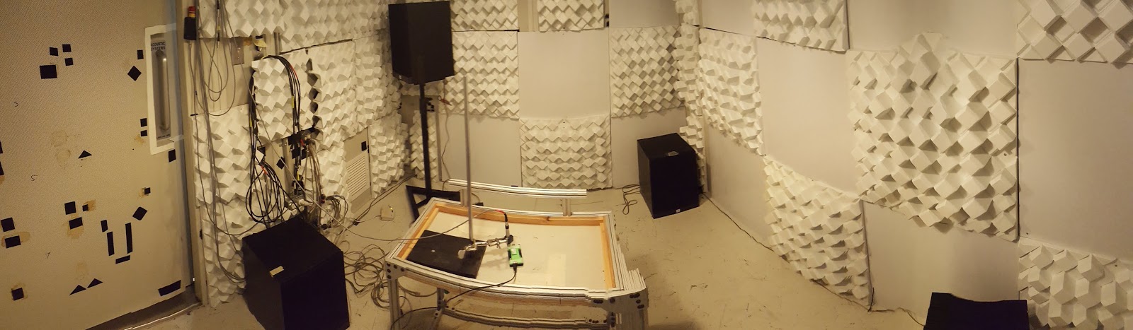
TEST SETUP

In addition to the Tympan Rev D and our HDA 200 headset, we used a Bruel & Kjaer Artificial Ear (4153) along with a Bruel & Kjaer microphone (4192). We used a LabVIEW data acquisition system to record the electrical signal produced by the Tympan and the microphone signal produced by the 4192 from the artificial ear.

TYMPAN FIRMWARE

We programmed the Tympan to produce sine test tones at different frequencies and amplitudes. The Tympan program is on our GitHub here

LABVIEW SOFTWARE

We used a laboratory-grade data acquisition system from National Instruments along with a LabView program to record our data. We recorded the microphone signal from the artificial ear and, per ANSI-ASA-S3.6-2018 (Section 6.1.5), we also recorded the electrical signal produced by the Tympan itself. All data were recorded as WAV files at a sample rate of 96 kHz.

COLLECTING DATA

After placing the headset on the artificial ear, we would command the Tympan to play a steady tone at the desired frequency. We would record the output of the Tympan and of the artificial ear.  We would then increment the amplitude and/or frequency and repeat the recording. All data were post-processed using these Matlab scripts.

DISTORTION LIMITS

For this test, we define the maximum sound pressure level (SPL) to be the highest level produced by the headset when the harmonic distortion is still below our limits. Using ANSI-ASA-S3.6-2018 (Section 3.1.5) as a reference, we set our distortion limits to be:

• No more than 2.5% total harmonic distortion
• No more than 2.0% distortion for the second and third harmonic
• No more than 0.3% distortion for the fourth and each higher harmonic

Continuing to take inspiration from S3.6-2018, we assessed the harmonic distortion using the microphone signal for the tones below 6 kHz while, for the tones at 6 kHz and above, we assessed the harmonic distortion using the electrical signal recorded directly from the Tympan.

RESULTS: Sound Pressure Level

The table and figure below show the maximum SPL that we achieved at each test frequency while staying within the distortion limits defined above.

RESULTS: Hearing Level

In addition to reporting the maximum values as sound pressure level (SPL), it is often desired to know the values expressed as “Hearing Level” (HL). HL can be computed from SPL given the “reference equivalent threshold sound pressure level” (RETSPL) that is provided by the headset manufacturer.  The RETSPL values for the Sennheiser HDA are published and were included in the table above.  As a result, the maximum HL that can be produced by the HDA 200 as driven by the Tympan are shown in the table and in the figure below.

DISCUSSION

Overall output level.For the commonly used audiogram frequency range (125–8000 Hz), the Tympan with the HDA200 can produce up to 108–115 dB SPL (or 79–105 dB HL), depending upon the specific frequency of interest.

Decreasing SPL at Higher FrequenciesIn the extended high frequency range (> 8kHz), we see that the maximum SPL drops modestly as frequency increases. This modest drop is due to the frequency response of the HDA200 headset; the voltage/current provided by the Tympan in this frequency range is consistent with the lower frequencies.

Decreasing HL at Higher Frequencies. Of course, when looking at the HL values at the extended high frequencies (> 8 kHz), the maximum HL values drop dramatically, but this result is due to the lower sensitivity of human hearing at these frequencies and is not related to the performance of the headset or of the Tympan.

Potential Level with Other Headsets. This testing only evaluated the maximum level of the Tympan when used with the HDA200. If the Tympan is used with other headsets, different maximum level values should be expected. For example, we tested the Tympan with consumer earbuds (see here) and saw loudness values of 105-117 dB SPL at 1 kHz, depending upon one's distortion criteria.

Tympan’s Electrical Output. The Tympan provides an electrical signal to drive the headset. It is the headset that converts the electrical signal into acoustic level. Regardless of frequency, the Tympan’s hardware is designed to deliver a clean output up to an amplitude of approximately 1 Vrms into a load of at least 32 ohms.  So, if you need more loudness than seen here with the HDA200, you can easily try your own favorite headset or earphones!

What Triggers Audio Processing?

Using the Teensy or Tympan for audio processing can be very exciting.  It's really fun to open up the example programs, compile them, and listen.  It's also pretty easy to look at the example code to see how the algorithm blocks are created and connected together.  Great!  But, what if you want to make your own algorithm?  That's when start to look a bit more critically at the examples.  Your first thought will likely be: "Wait.  How does any of this audio processing actually get called? How does this crazy structure work?!?"   Yes.  That's a good question.  Let's talk about it.

So Much is Hidden.  The essential problem is that nearly all of the audio plumbing is hidden so that its complexity doesn't scare people off.  For example, look at an extremely minimal audio processing example in the image below.  It instantiates the audio objects and creates the audio connections.  Then, you've got the traditional Arduino setup() and loop() functions.  Note that the loop() function is empty.  This program looks like it does nothing.  Yet, audio does flow.  The audio is made louder by the gain block applying 6 dB of gain.  But how?!?  I see no functions that call into the audio blocks!

What You Didn't Know That You Programmed.  The screenshot above shows the code that you know that you programmed.  There is also a whole bunch of code that you included, however, that you didn't know that you were invoking.  In effect, you programmed some very complex activities and you didn't even know it.

Going Down the Rabbit Hole.  The flow chart below tries to expose some of the hidden code.  This is a map that helps explain some of the hidden underground parts of the Teensy Audio Library (and Tympan Library). 

1) Code Shown in the Arduino Window.  The blocks in blue are the pieces of code that you know that you wrote.  This is the code shown in the Arduino IDE.  Here, you instantiate the audio classes and the audio connections.   Here, you write the Arduino setup() and loop() functions.  This is the part that we can all see and (usually) understand.  For the audio processing, the hidden magic gets invoked behind the scenes by the audio classes.  In particular, the AudioOutputI2S class is the most magical.

2) Audio Class Constructors.  As a bit of background, "I2S" is a communication system built into the Teensy processor that is purposely design to pass sound data (that's the 'S' in I2S) between the processor and the audio input/output hardware.  So, the AudioOutputI2S class handles the passing of audio data out from the processor to the audio output.  If you were to open the AudioOutputI2S class, you would see that its constructor calls its begin() method.  Looking in begin(), you'll see that it configures the I2S bus (which is logical) but it also configures the DMA and it attaches an interrupt to the DMA.  Huh?

DMA. Direct Memory Access is a special way of using memory.  You know how you can drive your car and listen to a podcast at the same time?  Your brain is able to handle certain tasks autonomously in the background without disturbing the foreground thoughts?  The processor has some of the same capabilities.  The processor can allow for certain regions of its built-in memory to be directly accessed by external devices.  In this case, DMA is configured so that the audio output system can read audio data directly from the processors memory without the processor having to respond to a request for each and every sample.  That's DMA.  It happens in the background.

3) Firing an Interrupt (ISR).  When the DMA is set up, it's pointed to a small region of memory.  The region holds a fixed number of audio samples.  Once the I2S bus is commanded to begin pumping data, it starts pulling data from the DMA.  Again, this happens in the background.  As the DMA empties, it'll get low on samples that remain.  In the DMA setup, the DMA has been configured to call a function (an interrupt service routine, ISR) to replenish the data in the DMA.  In the AudioOutputI2S begin() method, a specific function was attached as the ISR.  You didn't know it, but it was.  The ISR is right there in AudioOutputI2S.

Interrupting All Other Activities.  When the ISR is requested, the processor now has to take notice.  It is called an "interrupt" service routine because it interrupts whatever else is happening.  Whatever else the processor is doing (such as looping around in your Arduino loop() function) will be paused while the processor goes off and executes the ISR.  This interruption is done so that we can ensure there is fresh audio data placed into the DMA before the DMA fully empties and the audio stalls.

4) Execute the ISR.  Looking in AudioOutputISR, we see that the ISR copies previously-processed audio data into the DMA.  This keeps the DMA fed so that there are no hiccups in the audio.  Great.  The next thing that the ISR does is command update_all(), which starts the audio processing chain so that processed audio will be available the next time the DMA is running low.  This update_all() is the key.

Doing the Audio Processing.  The update_all() method lives in AudioStream.  AudioStream is the root (parent) class of every audio processing class that you might have instantiated in your Arduino code.  AudioStream has some static data members that, in effect, act as a central location for tracking every audio processing object that needs to be called.  Update_all() simply loops through the list of your audio objects and calls each one's update() method.  

Each Class's Update().  If you open up any audio class, you'll find that there is an update() method.  This is where all the audio processing is done.  Inside the update(), it pulls blocks of audio from its upstream connections and pushes audio blocks out to its downstream connections.  These upstream and downstream connections are known because of you created them in your Arduino code via those AudioConnection lines.

Summary.  So, that's how the audio processing happens on Teensy (and Tympan).  There is the code that you explicitly wrote and then there is all the code that comes along with the libraries, such as the class  AudioOutputI2S.  AudioOutputI2S sets up the I2S bus for passing data to the audio hardware and it sets up the DMA for feeding data to the I2S bus.  Whenever the DMA gets low on data, it fires an ISR.  The ISR refills the DMA and it launches the cascade of update()for all your audio objects.  Because it is interrupt driven, it all happens in the background...and that's why your Arduino code looks so empty.

Phew.  Good work, everyone.

Formant Shifting with Tympan

Once you have a real-time platform for manipulating audio, it is always fun to see what you can do to your voice.  In my case, I had been spending a lot of time figuring out a good way to implement frequency-domain audio processing on the Tympan.  Once I did that, I realized that it would be super easy to start having fun with my voice.  So, here, I present my Tympan Formant Shifter!

Formants vs Pitch.  Like any instrument, your voice has a pitch, which is the fundamental frequency of the sound of your voice.  The sound of your voice contains many harmonics, in addition to the fundamental frequency.  Those harmonics extend upward far above the fundamental frequency.  Which of those harmonics are actually projected from your mouth depend up how your mouth (and nasal passages and throat) are shaped.  As you talk, you naturally change the shape of your mouth (and nose and throat) to make the various consonant and vowel sounds.  An "E" sounds different from an "A" because your throat/nose/mouth enhance different harmonics for the two different vowels.  These enhanced frequency regions that move around -- these are your "formants".  

Formant Shifting.  In the video, I am only moving the formants.  Clearly, the effect on us listeners is that we feel like my voice itself is going higher or lower.  But, this isn't the case.  The fundamental frequency of my voice and the frequencies of the harmonics are all unchanged.  Instead, the formant shifting allows you to hear harmonics of my voice that are higher than your normally hear or lower than you normally hear.  The processing is shifting which harmonics are emphasized or attenuated.

Frequency-Domain Formant Shifter.  A formant shifter is implemented easily in the frequency domain.  Starting from your audio, take an FFT, shift the magnitude of the FFT bins to higher or lower bins (while leaving the FFT phases in their original bins), take the inverse FFT ("IFFT"), and play the audio.  In principle that's it!

Real World FFT/IFFT Processing.  In reality, of course, implementing the FFT/IFFT processing on a real-time audio stream is more complicated.  But, as I said at the top, I took quite a bit of time to try to hide all of these complications.  It takes care of the buffering, the windowing, and the overlap-and-add operations.

Tympan Example Code.  In the Tympan Library, I wrote an example sketch for Formant Shifting.  You can see it here.  The underlying audio processing class that does the formant shifting is here (*.h) and here (*.cpp).  Finally, for the video at the top, I combined the Formant Shifting with a USB Audio interface so that it would get recorded along with the video from my web camera.  You can get this USB Audio enabled version of the code (along with other partly-working goodies) here.

More Frequency-Domain Examples.  Once I got the whole frequency-domain processing structure in place, I found it fun and easy to implement several other frequency-domain algorithms.  In addition to Formant Shifting, I've got Frequency Shifting (but it is only linear shifting, not exponential scaling).  I've also got Frequency Compression and Noise Reduction.  I totally nerd-ed out.  So fun!

Tympan at High Speed (Ultrasonic!) Sample Rates

While we designed the Tympan as a platform for trying hearing aid algorithms, it's flexible enough to be used for many different audio tasks.  For example, by increasing the Tympan's sample rate, you can see signals above the range of human hearing...to explore ultrasound!  The question is, how high into the ultrasonic range can the Tympan go?

Sample Rate and Nyquist.  The Tympan is a digital audio device; it samples the voltage of a signal at discrete moments in time.  It acquires audio samples at a constant rate, the "sample rate".  If you wish to sense a certain frequency of audio (say 10 kHz), you need a sample rate that is fast enough to capture this frequency.  Thanks to Nyquist, we generally say that the sample rate needs to be at least twice the frequency of the signal that you want to sense.  So, to sense 10 kHz, our sample rate must be *at least* 20 kHz.  Typically, digital audio systems run at 44.1 kHz or 48 kHz so that they can comfortably span the 20 kHz maximum range of human hearing.

//set the sample rate and block size
const float sample_rate_Hz = 48000.0; //for audible sound
const int audio_block_samples = 128; 

Ultrasound.  For sensing ultrasound, we need to sense frequencies higher than 20 kHz.  Many inexpensive ultrasonic range-finders, for example, operate near 40 kHz.  If we want to explore these signals, we need to increase our sample rate to 80+ kHz.  Some rats and bats make vocalizations that extend up to 80 kHz, so that would require a sample rate of 160+ kHz.  Can the Tympan sample this fast?

Changing the Sample Rate.  Changing the sample rate of the Tympan is easy.  Near the top of every Tympan example, you can see where to change the sample rate.  This example is even called "ChangeSampleRate".  So, that part is easy; simply write in a sample rate that is higher!  The question is whether the Tympan produces useful data when running at these higher speeds.  Let's test it!

//set the sample rate and block size
const float sample_rate_Hz = 96000.0; //for ultrasound
const int audio_block_samples = 128; 

Test Setup.  As shown in the photo at the top of this post, I used a function generator to make a sine wave.  I then ran its signal through an attenuator to make sure that I wasn't overdriving the input of the Tympan.  I used a Tympan RevE and inserted the signal via its pink input jack.  

Tympan Software.  On the Tympan, I used one of the example sketches that records audio to the SD card.  In the code, I made two changes: (1) I told it to record from the pink jack as line-in and (2) I changed the sample rate to whatever I was testing.

Test Method.  For each test, I started the Tympan's SD recording and then I manually turned the knob on the function generator to sweep up through the frequency range.  I then stopped recording, pulled out the SD card, and made a spectrogram of the recording on my PC.  I used Matlab, but you could also use Python or Audacity for your spectrograms.

Results, Clean Audible Signal (fs = 48 kHz).  I started with a known-good traditional audio sample rate.  The figure below shows my frequency sweep when using a sample rate of 48 kHz.  The spectrogram shows that we could see frequencies up to 24 kHz, as expected based on Nyquist.  The spectrogram looks great; the signal is clean and the background noise looks like background noise.  This is what "clean" and "good" look like.

Results, Clean Ultrasound Signal (fs = 96 kHz).  I then turned up the sample rate to 96 kHz and repeated the measurement.  The spectrogram below is the result.  It looks great.  We see our signal up to 48 kHz, as expected.  There's a little bit of aliasing as the input signal continued past 48 kHz (we see that the signal's line in the spectrogram bounces downward a little bit when it hits 48 kHz).  The aliasing stops quickly, so this seems fine.  I think that this spectrogram looks great.

Results, Marginal Quality (fs > 96 kHz).  When I increase the sample rate beyond 96 kHz, the results start to look less good.  Below are the results for 100 kHz, 105 kHz, and 110 kHz.  As you can see, the signal itself looks OK, but strange artifacts start to appear in the background noise.

Results, Bad Quality (fs > 110 kHz).  Finally, by the time we get to a sample rate of 115 kHz, the recorded audio is bad.  Bascially, any sample rate above at 115 kHz and above is unusable.

Conclusion.  The Tympan is good for recording at sample rates up to 96 kHz.  You can maybe even run up to 110 kHz.  But, at 115 kHz and above, your signal will be corrupted.

Improving High-Frequency Performance.  The audio codec used to do the sampling is a very complicated device.  There are many settings and many ways of clocking the device.  It is possible that there is a different combination of settings that would provide good-looking data at sample rates higher than 96 kHz.

96kHz is Still Good!  Luckily, 96 kHz is still a very useful sample rate for ultrasound.  Running at 96 kHz is fast enough to give good access to signals around 40 kHz.  This is a very important region for ultrasound in air.  There are many ultrasonic range finders and motion sensors that operate in the 40 kHz range.  So, you can explore and do many fun things running your Tympan at 96 kHz.  Furthermore, we also know that the Tympan's on-board microphones are sensitive up into this region, so you don't even need any additional hardware to sense the ultrasound!  You can just change the system's sample rate and then go have fun!

Microphone Self-Noise (Tympan Rev-D2)

As mentioned in a previous post, it is important for hearing aids that the microphones and electronics have a low self-noise.  Because of the amplification in a hearing aid, what might start as an innocuous amount of noise gets multiplied into a very annoying and fatiguing listening experience.  So, for our next revision of Tympan (Tympan Rev-D2), we're looking to further reduce the self-noise of the system.  We are considering an on-board microphone that should offer 5dB less self-noise than the existing design (Tympan Rev-C).  Instead of taking their word for it, let's place the Tympan mics in a super quiet room and see what happens.

Backstory:  The current release of Tympan is "Rev-C".  It is a fine system, though a bit bulky.  Rev-C is bulky because it is composed of two separate boards: the Teensy 3.6 and the Tympan audio board.  To reduce the bulk, we've smashed them together into one board.  This is our new "Rev-D".  The first version (Rev-D1) is otherwise identical to Rev C -- it has the same on-PCB microphones and the same audio interface.  It appears to have the same performance as Rev-C, which is what we expected.  With that success, we're now trying to further improve the system by focusing on its self-noise.  That's Rev-D2.  For Rev-D2, we're using quieter on-PCB microphones and we've added an additional (hopefully even quieter) pre-amplifier for the mics.  We'll see!

Goal:  Today's goal is to compare the self-noise of the new Rev-D2 to the existing Rev-C/Rev-D1.  We expect to see that D2 is quieter, primarily due to its quieter on-PCB microphones.  From the datasheet specs (below), the proposed mic should offer a significant reduction in self-noise (-5dB) (measured at 1kHz), compared to the existing mic.  While comparing Rev-D2 to Rev-C/Rev-D1, we'll also compare to a laboratory grade reference microphone from B&K.

Design	Microphone	Mic Sensitivity dBV/Pa	Self-Noise (dBA)
Existing Mic (Rev-C/Rev-D1)	Knowles  SPH1642HT5H-1	-38 @ 1kHz	29
Proposed Mic (Rev-D2)	Knowles  SPM0687LR5H-1	-32 @ 1kHz	24
Reference Mic	B&K 4191	-38 @ 250Hz	20

Setup

Approach: The first step is calibrating each Tympan's microphone so that we know how to interpret the recorded audio.  By calibrating each Tympan's microphone, we can express the apparent self-noise levels in terms of apparent sound pressure level (SPL), which is a good way of doing an apples-to-apples comparison across systems.  After we've calibrated the Tympan systems, we'll put the Tympan's into a quiet sound room to (hopefully) measure their self-noise.  Ideally, the ambient noise in the sound room will be low enough to discern the self-noise of the on-board microphones.

Hardware:  We used a Tympan Rev-D1 and a Rev-D2.  We also recorded the ambient sound levels using our laboratory-grade reference microphone, a B&K 4191 along with a National Instruments data acquisition system.   

Gain Settings: In addition to the new microphone on Rev-D2, the Rev-D2 also features a new preamp between the microphone and the Tympan's audio interface chip (a TI AIC3206).  The pre-amp provides about 15 dB of additional gain via an amplifier that we believe to be quieter than the programmable gain in the AIC3206.  Therefore, for the testing with the Rev-D2, we turned down the gain on the AIC3206 by 15 dB, which should make the overall gain between the Rev-D1 and Rev-D2 about the same.  

Physical Setup: The sound recordings were made in a single-walled, acoustic test chamber, which is fairly quiet above  125 Hz.  As shown in the figure at the top of this post, the lab-grade B&K microphone was positioned 1" above the Tympan's on-board PCB mic so that it is placed along the same axis as the mic under test.  

Tympan Setup.  The Tympans were configured to record from their on-PCB microphones.  They were configured to use a sample rate of 44.1 kHz and to write their raw audio data straight to the Tympan's SD card.  The Tympan Arduino code is here on GitHub.  The Tympans were running on their battery power.

Calibration

To calibrate the microphones across a wide frequency spectrum (125Hz-22kHz), white noise was created in an audio effects editor and played through 4 speakers in the sound room.  The speakers were pointed in different directions to create a diffuse, rather than directional, sound field.

To define the Tympan's frequency response from 125Hz to 16kHz, the Tympan output was filtered by octave-bands, then the RMS value was taken and converted to a dB log scale that references the Tympan's Full Scale Output (+1.0).

Sensitivity for a digital microphone is often reported as the output at 94dB SPL (i.e. 1 Pa), compared to its full-scale output:

This sensitivity can be rephrased in terms of the dB log scale:

The figure below shows the raw microphone response and the derived sensitivity.  At 1kHz, the proposed microphone (D2) is less sensitivity (-1.8dB) than the existing microphone (D1), which is expected.

Self-Noise

Now that the microphones are calibrated, we can take a recording of a quiet sound room with the mics under test and relate that to an equivalent sound pressure level.  The same analysis was applied as before: the recording was filtered into octave bands then the RMS value was taken for each band.

From the figure below, the proposed mic shows a 1.5dB reduction in self-noise at 1kHz, compared to the existing mic.   We can also report the A-weighted average by applying a correction to the RMS value for each octave band (as described here).  That shows a 1.7dB reduction in A-weighed self-noise.

Conclusion

The self-noise of the proposed microphone offers a small improvement in self-noise (2dB) which is less than that expected from the datasheets (5dB).  As a follow-up, it will be interesting to see if this is due to the thermal noise of the microphone, or self-noise in the front-end electronics.

Microphone Self-Noise

A hearing assistive device must not be noisy.  At minimum, noise will be annoying.  At worst, noise will harm, not help a person's ability to hear.  So, for our Tympan device, I want to make sure that it has low self-noise.  In this post, I show how the microphone that you choose can strongly affect the apparent noise of your system.  Spoiler: be careful with lapel mics because they can be very noisy!

Goal:  I want to measure the self-noise of different microphones in combination with the Tympan.

Approach:  My approach is to first calibrate the Tympan when using each microphone.  That way, when comparing between microphones, I'm comparing apples-to-apples.  Once calibrated, I will put the devices in a super-quiet environment and make ambient sound recordings.  The super-quiet environment will probably be so quiet that recordings will reveal the self-noise of the microphones.

Hardware:  As shown in the picture above, I am testing with a Tympan Rev C, which includes built-in microphones (Knowles SPH1642) on its PCB.  I also made recordings with a Sony lapel microphone (ECM-CS10) plugged into the Tympan's microphone jack.  As a reference microphone for the calibration, I used a B&K 2250 sound level meter (SLM) with its 4191 microphone element.

Setup:  I performed the recordings in our single-walled acoustic test chamber in the basement of our building.  It is fairly quiet, though it is not as quiet at the lowest frequencies (125 Hz and below).  As shown in the figure at the top of this post, I put the lapel microphone and the B&K microphone very close to the Tympan's built-in PCB mic.

Device Configuration:  The Tympan was configured to record audio straight to its SD card as 32-bit floating point samples, switching automatically between the two microphones after a fixed interval of time.  It was configured with an input gain of +15dB for all recordings.  My code is on GitHub here.  The B&K SLM was configured to record its calibrated audio to its compact flash card.

Calibration:  To calibrate the microphones, I played white noise into the sound chamber.  The B&K SLM recorded the audio in calibrated units, as shown in the first plot below.  Simultaneously, the Tympan recorded the audio (through each of the two microphones) in uncalibrated units, as shown in the second plot below.  By comparing the raw Tympan levels with the calibrated B&K levels, the bottom plot shows the sensitivity of the Tympan+microphone at each frequency.

Measuring Self-Noise:  Turning off the white noise stimulation, the sound chamber was very quiet. Again, the B&K SLM and the Tympan made recordings from their microphones.  My assumption is that, especially for the Tympan, the true background noise in the sound chamber was so low that the recordings will reveal the self-noise of the microphones.

Self-Noise Expressed as SPL:  The first plot below shows the raw, uncalibrated noise levels recorded by the Tympan.  To convert these values to SPL, I need to apply the calibration data discussed above.  There's a couple ways that I could apply the calibration.  The middle plot shows the estimated SPL if I were to have calibrated the Tympan only at a 1 kHz, which is a common, simple way to calibrate a device.  Alternatively, if we use the full frequency-dependent calibration for the Tympan, the bottom plot shows the estimated SPL.  Using either calibration approach, the conclusion is the same: the Sony lapel mic has much higher self-noise than the built-in PCB mics!

The Microphone Matters!  Getting quantitative, I can summarize these spectra by applying an A-weighting curve and computing the broadband sound pressure level (ie, "dBA").  From these recordings, the Tympan + Lapel Mic has a self noise equivalent to an ambient noise level of 41-43 dBA (depending upon the calibration approach).  By contrast, the Tympan + PCB Mics show a noise level of between 27-29 dBA.  This 14 dB difference is a big!

Conclusion:  Since low self-noise is good, the Tympan's built-in PCB microphones seem to be a better choice than this Sony lapel microphone.  I look forward to trying other microphones to see if I can get even lower self-noise.

Follow-Up: What Self-Noise Should Be Expected?  After completing this post, I realized that I should have looked at the microphone datasheets to see what the manufacturers say about each microphone's self-noise.  Here's what I found:

• For the PCB mics (SPH1642), the self-noise is not reported directly.  But, they report the signal-to-noise ratio as 65 dBA when given a 1 kHz signal at 94 dB SPL.  This means that the noise floor for the mics is (94 dB - 65 dBA) = 29 dBA.  This is exactly the value that I found, when I used the simple calibration for 1 kHz.  This gives me additional confidence in my measurement technique.
• For the Sony lapel mic (ECM-CS10), the noise level is reported simply as "38 dB".  Presumably, this is A-weighted, but there is no more information provided.  My own value (41 dBA, for single-frequency calibration) is 3 dB higher than the datasheet value.  The cause for the difference is unknown, though the difference is modest.

Measuring Audio Latency

For real-time audio processing, it is often important to minimize the delay between audio coming out of the system compared to the audio coming into the system.  This is especially true of hearing aids, where too much latency can cause the listener to perceive an echo (or have a comb-filtering effect), which end up degrading rather than helping the listener's experience.  Research suggests that the maximum tolerable latency in a hearing aid is only 14-30 msec.  If Tympan wants to be helpful, we need to make sure that we keep our latency shorter than this.  Let's find out what our system does!

Test Setup.  To measure the latency of the Tympan, we need to inject an audio signal into the Tympan and then measure delay of the output audio relative to the input audio.  There's lots of ways that this can be done.  I chose to use the setup shown in the picture above.  In this setup, I generate my test audio signals from my PC.  I use a series of 1 kHz tone bursts that are 1 second long.  The audio comes out of my PC and (as shown in the red line) is split so that it goes to the input of the Tympan *and* to the input of an audio recorder.  The output of the Tympan is then (as shown in the blue line) routed to the other input of the audio recorder.  The stereo audio file produced by the audio recorder will contain the input audio in the left channel and the output audio in the right channel.  It will then be a simple post-processing analysis to measure the delay between the two channels.

Raw Data.  An example recording and an example Matlab processing script are in my GitHub here.  The plot above shows the example data.  As you can see, there are three tone bursts in the recording.  At this timescale, one cannot see any delay between the signals, but that is because we are not zoomed in enough.  The plot below zooms in to the start of one of the tone bursts.  Here, we definitely see that the Tympan output has a slight delay relative to the direct audio signal.

Analysis.  Using the plot above, we could visually assess the latency between the two channels.  But, to do even better, I included a Matlab script in the GitHub directory that computes the cross-correlation between the two channels.  The best estimate of the latency will be when when the cross-correlation is maximum.  For this recording, the best estimate of the latency is 3.1 msec.  That's nice and short!

Measuring other Tympan Configurations.  Expanding from this single measurement, I then repeated the process and measured the latency for a variety of different configurations of the Tympan.  I tried different audio block sizes and I tried different audio processing algorithms.  My results are shown in the figure below.  The simple 3.1 msec value reported above can be seen in the bottom-left of the plot as the first point on the yellow line.  All of the other configurations result in increased latency, but there are still a lot of configurations that are shorter than the 14-30 msec upper limit from the literature.

Components of the Latency.  After working with the system for a while, I've identified three contributors to the latency:

• Hardware:  The audio interface for the Tympan is a TI 3206 AIC.  This chip has a pipeline that is 17 samples long on the input and 21 samples long for the output.  So, for this round-trip testing, it contributes 38 samples of latency, which at sample rate of 24 kHz is a latency of 1.58 msec.
• Audio Library:  The Tympan audio library is based on the Teensy audio library, which has employs a queue of two audio blocks in order to prevent audio hiccups and drop-outs.  In the Tympan library, this audio block size is configurable, hence my ability to make the graph above where I vary the block size.  For a block size of 16 samples, the library's latency is 2*16=32 samples, which is 1.33 msec at 24 kHz.  Totaled with the hardware latency (1.58 msec + 1.33 msec), we get 2.9 msec, which is very close to the 3.1 msec value that I measured.  Great!
• Audio Processing:  Beyond the audio library, most any actual audio processing will also introduce additional latency.  A typical (symmetric) FIR filter, for example, will result in a group delay that is half the length of the FIR filter.  Other filters and other operations (such as FFT) introduce delays as well.  The specific amount of latency may vary, but some latency is inherent in the math.  For the Tympan, we see the latency for FIR and FFT in the graph above.

Optimizing for Minimum Latency.  From this exploration, I've learned that latency can be minimized by (1) using the shortest audio block size that the system can handle and (2) running the simplest audio processing algorithm that you can get away with.  On this latter point, we all want our audio processing to have extremely fine frequency resolution.  But, high resolution requires long FIR filters or long FFTs.  Long FIRs/FFTs introduce a lot of latency, however.  So, if you want low latency, you need to use the shortest FIRs and FFTs that you can.